Conformal Prediction with Upper and Lower Bound Models

By Miao Li, Michael Klamkin, Mathieu Tanneau, Reza Zandehshahvar, and Pascal Van Hentenryck (Georgia Institute of Technology)

link: https://www.arxiv.org/abs/2503.04071

Part 1: Author's Summary

(1) A: Welcome everyone to today's lab meeting. We have a presentation from the authors of "Conformal Prediction with Upper and Lower Bound Models." The lead author will give us a 7-minute overview of the paper, after which we'll open the floor for questions. Please, go ahead.

(2) Author: Thank you for the opportunity to present our work today. Our paper introduces a new approach to uncertainty quantification in regression problems, specifically in settings where we have deterministic upper and lower bounds on the target variable.

Let me set the stage. In many real-world applications, particularly in optimization problems, we often can compute valid upper and lower bounds for a quantity of interest. For example, in parametric optimization problems, we can derive lower bounds from dual-feasible solutions and upper bounds from primal-feasible solutions. These bounds are valid by construction, meaning the true value is guaranteed to lie between them. However, these bounds can sometimes be too conservative, making them less useful for decision-making.

What we propose is a method to tighten these bounds while maintaining a desired level of probabilistic coverage. The key insight is that by accepting a small reduction in coverage probability—say from 100% to 95%—we can substantially reduce the width of prediction intervals, making them much more informative for downstream tasks.

Our approach, which we call CPUL (Conformal Prediction with Upper and Lower bounds), has three main contributions:

First, we formulate a new setting for Conformal Prediction where only valid upper and lower bound models are available instead of the usual mean prediction model.

Second, we develop the CPUL algorithm that leverages multiple nested interval construction methods. This algorithm selects the best method based on empirical performance on a calibration dataset.

Third, we identify and address a paradoxical issue: in regions where the initial bounds are very tight, standard conformal methods tend to produce empty prediction intervals, leading to undercoverage. We introduce an Optimal Minimal Length Threshold (OMLT) mechanism to fix this problem.

Our method works as follows: We start with deterministic upper and lower bounds, then compute quantiles of the residuals between the actual values and these bounds. Using these quantiles, we construct four different families of prediction intervals. Through a model selection approach, we choose the family that delivers the smallest average interval width while maintaining the desired coverage level.

We validated our approach on large-scale energy systems optimization problems, specifically on bounding the optimal value of economic dispatch problems across different power grid datasets. The results show that CPUL and CPUL-OMLT consistently outperform baseline methods, producing tighter intervals while maintaining the target coverage.

Importantly, our approach doesn't require training any additional models—it works directly with the available bound models, making it computationally efficient. And unlike some existing methods, CPUL adapts to varying levels of heteroscedasticity between the upper and lower bound residuals.

To summarize, our work provides a novel approach to uncertainty quantification when valid bounds are available, delivering more informative prediction intervals that can significantly enhance decision-making in optimization problems. The approach is especially valuable in areas like power systems, investment analysis, and policy optimization, where tight yet reliable bounds on optimal values are critical. [Sections 1-6]

Part 2: Initial Discussion Round

(3) Junior: Thanks for the presentation. I'm still trying to understand what conformal prediction actually is. Could you explain it in simple terms for someone who has never worked with it before? What does it mean to have "95% coverage" in this context? And could you walk through the key equations step by step?

(4) Author: I'd be happy to explain conformal prediction from the ground up.

At its core, conformal prediction is a framework for creating prediction intervals with statistical guarantees. Let me break it down with an example:

Imagine you're trying to predict house prices. Instead of just predicting that a house will sell for $300,000, you want to provide a range, like [$280,000, $320,000], and you want to be confident that the true price will fall within this range with high probability.

"Coverage" refers to how often our prediction interval contains the true value. When we say "95% coverage," it means that if we make predictions for 100 different houses, the true price should fall within our predicted range for approximately 95 of them.

What makes conformal prediction special is that it provides this coverage guarantee without making assumptions about the underlying data distribution. It works with any prediction model and adapts the width of the prediction interval based on the uncertainty in different regions of the input space.

Here's how it works step by step:

1. We split our data into a training set and a calibration set.
2. We train our prediction model on the training set. Let's call this model f_hat. For a given input x, f_hat(x) gives us a point prediction.
3. For each example (x_i, y_i) in the calibration set, we compute a "nonconformity score" which measures how different the true value y_i is from our prediction f_hat(x_i). A common choice is the absolute error:s_i = |y_i - f_hat(x_i)|where y_i is the true value and f_hat(x_i) is our prediction.
4. We find the (1-α) quantile of these nonconformity scores, where α is our desired error rate (e.g., α = 0.05 for 95% coverage). Let's call this quantile q.
5. For a new input x_new, our prediction interval is:[f_hat(x_new) - q, f_hat(x_new) + q]

This interval will contain the true value y_new with probability at least 1-α, assuming the data is exchangeable (a weaker assumption than independence).

In our paper, we modify this framework because instead of having a single prediction model f_hat, we have two models:

• A lower bound model B_l that always gives values below the true value
• An upper bound model B_u that always gives values above the true value

So for any input x, we already have a valid interval [B_l(x), B_u(x)] with 100% coverage. The problem is that this interval might be too wide to be useful.

Our goal is to shrink this interval while maintaining a desired coverage level, like 95%. We do this by applying the conformal prediction framework to refine these bounds.

Does this explanation help clarify what conformal prediction is and what we mean by coverage? [Sections 2, 3]

(5) Junior: Yes, that's much clearer! So you start with bounds that are 100% certain but possibly too wide, and you're willing to accept a small chance of error to make them narrower. But how exactly do you shrink the interval using conformal prediction when you already have these bounds?

(6) Author: Exactly right! Now let me explain how we shrink the interval step by step.

When we have deterministic upper and lower bounds, we know that for any input x: B_l(x) ≤ true_value(x) ≤ B_u(x)

These bounds already give us a prediction interval with 100% coverage, but as you noted, this interval might be too wide to be practically useful.

Here's how we shrink it using our CPUL approach:

Step 1: We calculate how far the true values are from our bounds in our training data.

• For the lower bound, we compute the residuals: r_l = true_value - B_l(x) These residuals are always positive since B_l(x) is always below the true value.
• For the upper bound, we compute the residuals: r_u = true_value - B_u(x) These residuals are always negative since B_u(x) is always above the true value.

Step 2: We find certain percentiles (quantiles) of these residuals.

• For the lower bound residuals, we find the α/2 quantile (Q_l_α/2) and the 1-α/2 quantile (Q_l_1-α/2)
• For the upper bound residuals, we find the α/2 quantile (Q_u_α/2) and the 1-α/2 quantile (Q_u_1-α/2)

Where α is our target error rate (e.g., α = 0.05 for 95% coverage).

Step 3: We use these quantiles to define four adjusted bounds:

• L_l(x) = B_l(x) + Q_l_α/2
• L_u(x) = B_u(x) + Q_u_α/2
• U_l(x) = B_l(x) + Q_l_1-α/2
• U_u(x) = B_u(x) + Q_u_1-α/2

Step 4: We combine these adjusted bounds to create four different types of intervals:

1. [L_l(x) - t, U_l(x) + t] - using only the lower bound model
2. [L_l(x) - t, U_u(x) + t] - using lower bound for the left end, upper bound for the right end
3. [L_u(x) - t, U_l(x) + t] - using upper bound for the left end, lower bound for the right end
4. [L_u(x) - t, U_u(x) + t] - using only the upper bound model

The parameter t is a threshold that we calibrate to achieve our desired coverage level.

Step 5: We calibrate each of these four interval types on a calibration dataset and choose the one that gives the narrowest intervals while maintaining our target coverage.

The key insight is that by using the quantiles of the residuals, we're capturing how the uncertainty varies for different inputs. And by considering four different ways to construct the intervals, we can adapt to situations where one bound might be more accurate than the other.

Finally, we always intersect our calibrated interval with the original bounds [B_l(x), B_u(x)], since we know the true value must lie within these bounds.

Is that clear, or would you like me to elaborate on any particular step? [Section 3.2]

(7) Dr. P: Thank you for that explanation. I've been looking at Algorithm 1 in your paper, which outlines the CPUL method. If I understand correctly, the algorithm splits the dataset, trains bound models, computes empirical quantiles, forms four different interval constructions, and then selects the model with the smallest width.

What caught my attention is that you're selecting a single model from the four variants for the entire test set. Did you consider a more adaptive approach where the model selection happens on a per-sample basis? Also, what was the computational overhead of running four different calibrations versus a single calibration approach? I'm trying to understand the tradeoff between complexity and performance here.

(8) Author: You've summarized Algorithm 1 very well. You're right that CPUL selects a single interval construction (from the four variants) to use across the entire test set, rather than making this selection on a per-sample basis.

We did consider a per-sample selection approach, but we ultimately opted for a global model selection for several reasons.

First, selecting a model on a per-sample basis would require additional complexity to maintain the coverage guarantees. The theory for nested conformal prediction that we rely on applies most directly when using a single calibrated model across all test samples. Mixing different models for different samples would require additional theoretical guarantees that are non-trivial.

For example, if we naively chose the narrowest interval for each test sample without proper calibration, we would risk undercoverage because we would be essentially cherry-picking the most optimistic predictions.

Second, the global model selection is more computationally efficient during inference. Once we select the best model, we can simply apply it to all test samples without the overhead of making four predictions and then selecting the best one for each sample.

Regarding the computational overhead, running four calibrations instead of one does incur additional computation during the calibration phase, but this overhead is relatively minor for several reasons:

1. The calibration step is performed only once, not for every prediction.
2. The calibration process itself is very efficient - it essentially involves computing quantiles on the calibration set.
3. We don't need to train any additional models; we're just processing the residuals in different ways.

In our experiments, the calibration phase typically took just a few seconds even for our largest datasets with 5,000 calibration samples. This is negligible compared to the time required to train the original bound models (which is outside the scope of our method anyway).

The benefit of considering four different constructions far outweighs this small computational cost. As shown in Figure 3 of our paper, different constructions perform best on different datasets and for different coverage levels. Having this model selection capability allows our method to automatically adapt to the specific characteristics of the problem at hand. [Sections 3.2, 5]

(9) HoL: I appreciate how you're formalizing the problem. I'd like to better understand what you referred to as the "paradoxical miscoverage" issue. Could you explain this phenomenon in more detail? What exactly happens in those regions where the initial bounds are very tight, and how does your OMLT mechanism address this problem?

(10) Author: Thank you for asking about the paradoxical miscoverage issue. This is one of the most interesting and counterintuitive findings in our work.

To explain the paradox, let me first describe what happens in regions where our initial bounds are very tight - that is, where B_u(x) and B_l(x) are close to each other.

In standard conformal prediction, we typically add and subtract a constant value (let's call it t) from our point prediction to form a prediction interval. This constant t is calibrated on the entire calibration set to achieve our desired coverage level.

When we apply this approach with our bound models, we form intervals like [L_l(x) - t, U_u(x) + t], where L_l and U_u are adjusted versions of our lower and upper bounds.

Here's where the paradox occurs: In regions where the original bounds B_u(x) and B_l(x) are very tight (close to each other), our adjusted bounds L_l(x) and U_u(x) might also be very close, or even cross each other. When we apply the same constant adjustment t to these regions, we might end up with a situation where:

L_l(x) - t > U_u(x) + t

In this case, the resulting interval would be empty! And even when the interval isn't empty, it might be too narrow to contain the true value.

The paradox is that these tight regions are precisely where our original bounds are most accurate (they're already close to the true value), yet they're the ones most likely to suffer from undercoverage after calibration.

Let me illustrate with a simple example:

• In region A, B_u(x) - B_l(x) = 100 (wide bounds)
• In region B, B_u(x) - B_l(x) = 5 (tight bounds)

After calibration, we might add/subtract t = 30 to form our intervals. In region A, this gives a reasonable interval width of 100 - 230 = 40. But in region B, our interval becomes 5 - 230 = -55, which is nonsensical!

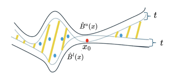
Figure 2 in our paper visualizes this issue. Around point x₀, the calibrated intervals don't cover the true value because the intersection of our adjusted interval with the valid region [B_l(x₀), B_u(x₀)] is empty.

Our OMLT (Optimal Minimal Length Threshold) mechanism addresses this by introducing a threshold ℓ that represents the minimum allowed length for a prediction interval. For any input x, if the gap between our bounds B_u(x) - B_l(x) is smaller than ℓ, we simply use the original bounds without attempting to tighten them.

Mathematically, we define: κ_ℓ(x) = the smallest t such that the interval width is at least ℓ

And then we construct our final interval as:

• If B_u(x) - B_l(x) ≥ ℓ and t > κ_ℓ(x): use the standard calibrated interval
• If B_u(x) - B_l(x) ≥ ℓ and t ≤ κ_ℓ(x): use an interval with minimum width ℓ
• If B_u(x) - B_l(x) < ℓ: use the original bounds [B_l(x), B_u(x)]

This approach guarantees that our prediction intervals have a minimum length of ℓ except in regions where the original bounds are already tighter than ℓ, in which case we simply use the original bounds.

The optimal value of ℓ is found by minimizing the expected interval width subject to the coverage constraint, which we solve using a grid search.

In our experiments, particularly on the 1354_pegase dataset, CPUL-OMLT effectively addressed the undercoverage issue in tight regions and produced overall tighter intervals compared to CPUL alone. [Section 4]

(11) Senior: I'm working on similar problems for my PhD, and I'm curious about how your method compares to existing approaches like Conformal Quantile Regression (CQR). From what I understand, CQR also adapts to different uncertainty levels in different regions of the input space. What would you say is the most novel aspect of your approach compared to these prior methods?

(12) Author: That's a great question about how our method relates to existing approaches, especially Conformal Quantile Regression (CQR).

You're right that CQR also aims to adapt to different uncertainty levels across the input space. Let me explain the key differences between our approach and CQR, and highlight what's novel about our work.

Conformal Quantile Regression typically works like this:

1. Train two quantile regression models to predict, say, the 5th and 95th percentiles of the conditional distribution.
2. Use these as initial prediction intervals.
3. Apply conformal prediction to calibrate these intervals to ensure valid coverage.

This is a powerful approach that can adapt to heteroscedastic noise (where uncertainty varies across the input space).

Our CPUL method differs in several important ways:

First, our starting point is fundamentally different. CQR requires training quantile regression models, which can be complex and data-intensive. In contrast, our method starts with deterministic upper and lower bounds that are already available in many optimization problems. We don't need to train any additional models beyond these bounds.

For example, in our power system application, the upper bounds come from primal-feasible solutions, and the lower bounds come from dual-feasible solutions to the economic dispatch problem. These bounds are valid by construction - the true optimal value must lie between them.

Second, CQR doesn't explicitly account for the asymmetric behavior between upper and lower bounds. Our CPUL framework constructs four different interval families that can adapt to situations where one bound might be significantly tighter than the other. This is particularly important in optimization problems where, for instance, the primal bound might be much tighter than the dual bound, or vice versa.

Third, we identified and addressed the paradoxical miscoverage issue that occurs in regions where the bounds are very tight. This is a novel insight that, to our knowledge, hasn't been addressed in previous work like CQR. Our OMLT mechanism provides an elegant solution to this problem.

In our experiments, both CQR and its variant CQR-r consistently performed worse than CPUL and CPUL-OMLT. As shown in Table 2 and Figure 3, they produced much wider intervals for the same coverage level. This is because they don't leverage the special structure of valid bounds.

To summarize the most novel aspects of our work:

1. We formulated a new problem setting for conformal prediction with valid upper and lower bounds, which is particularly relevant for optimization problems.
2. We developed the CPUL mechanism that integrates multiple interval construction strategies and automatically selects the best one based on empirical performance.
3. We identified the paradoxical miscoverage phenomenon and developed the OMLT mechanism to address it.
4. Our approach doesn't require training any additional models beyond the original bound models, making it computationally efficient and easy to apply in practice.

Does that help clarify how our work relates to and extends beyond existing methods like CQR? [Sections 2, 3, 4, 5]

(13) LaD: I'm interested in understanding the datasets you used for evaluation. Could you describe them in more detail? How were they created, what kind of distributions do they represent, and what makes them suitable for testing your method? I'm particularly curious about the size and complexity of these datasets.

(14) Author: I'm glad you asked about the datasets, as they're an important aspect of our evaluation.

We evaluated our approach on three power grid datasets of varying sizes and complexities:

1. 89_pegase: This dataset represents a portion of the European high-voltage transmission network with 89 buses (nodes), 12 generators, and 210 branches (transmission lines). The grid operates at voltage levels of 380, 220, and 150 kV.
2. 118_ieee: This is a standard benchmark in power systems engineering, modeling part of the American Electric Power system in the Midwestern United States as of December 1962. It contains 118 buses, multiple generators, and transmission lines.
3. 1354_pegase: This is our largest dataset, also representing part of the European grid but at a much larger scale. It contains 1,354 buses, 260 generators, and 1,991 branches operating at 380 and 220 kV.

The datasets come from established power system benchmarks. The pegase datasets are from the PEGASE project (Pan European Grid Advanced Simulation and State Estimation), which was part of the 7th Framework Program of the European Union. The ieee dataset is from the University of Washington's Power Systems Test Case Archive.

For our experiments, we didn't use the datasets as-is. Instead, we generated synthetic data points by varying the load patterns (electricity demand) across the grid. For each data point, we used the following procedure:

Each load d_l at location l was generated as: d_l = α × β_l × d_l^base

Where:

• d_l^base is the base load at location l
• α is a "global" scaling factor that affects all loads (sampled from Uniform(0.6, 1.0) for 89_pegase and 118_ieee, and from Uniform(0.8, 1.05) for 1354_pegase)
• β_l is a "local" scaling factor specific to location l (sampled from Uniform(0.85, 1.15) for all datasets)

This approach allows us to generate diverse but realistic load scenarios, reflecting how electricity demand varies in real-world grids.

For each dataset, we generated 50,000 data points, which we split into 40,000 for training, 5,000 for calibration, and 5,000 for testing. We repeated this process 10 times with different random seeds to ensure robust evaluation.

What makes these datasets particularly suitable for testing our method is that they represent real-world optimization problems where the concept of upper and lower bounds is naturally applicable. For each data point, we computed:

1. The true optimal value (ground truth) using an LP solver (HiGHS)
2. Upper bounds from neural network-based primal optimization proxies
3. Lower bounds from neural network-based dual optimization proxies

These datasets exhibit varying degrees of difficulty and characteristics:

• The bounds have different levels of tightness across different regions of the input space
• The accuracy of the bound models varies across datasets (as shown in Table 3 of our paper)
• The 1354_pegase dataset, being the largest and most complex, shows the most pronounced paradoxical miscoverage issue that our OMLT mechanism addresses

These properties allow us to thoroughly test the robustness and adaptability of our method across different scales and scenarios. [Section C.2 in Appendix]

(15) MML: I'm interested in the theoretical guarantees of your method. Looking at Theorem 2 in your paper, you provide a bound on the coverage probability. Could you walk us through this theorem in simple terms? What does this bound tell us, and how does it depend on the size of the calibration set? Also, is this a tight bound, or is it conservative?

(16) Author: I'd be happy to explain Theorem 2 in more accessible terms.

Theorem 2 provides the theoretical guarantee on the coverage probability of our CPUL method. It tells us that when we use Algorithm 1 to select the best interval construction, we can still provide a probabilistic guarantee on the coverage, despite the additional complexity introduced by the model selection process.

The theorem states:

P(Y_{N+1} ∈ C^{**}(X_{N+1})) ≥ (1+N_cal)/N_cal × (1-α) - η/√(N_cal)

Let me break down what this means:

1. The left side P(Y_{N+1} ∈ C^{**}(X_{N+1})) is the probability that our prediction interval contains the true value for a new test point.
2. N_cal is the size of our calibration set (the number of samples we use for calibration).
3. α is our target error rate (e.g., α = 0.05 for 95% coverage).
4. η is a constant approximately equal to 1.88, derived from concentration inequalities in probability theory.

The bound has two main components:

• (1+N_cal)/N_cal × (1-α): This part approaches (1-α) as N_cal gets large. For example, with N_cal = 1000 and α = 0.05, this is about 0.95095.
• η/√(N_cal): This part accounts for the additional uncertainty from model selection and decreases as N_cal increases. With N_cal = 1000, this is about 0.059.

So what this bound tells us is that as our calibration set size increases, our coverage probability gets closer to our target 1-α. But because we're selecting between multiple models, we need to pay a small "price" in terms of coverage, which is captured by the second term.

To give you a concrete example, with a calibration set of size N_cal = 5000 (as in our experiments) and targeting 95% coverage (α = 0.05), the bound guarantees approximately:

(1+5000)/5000 × 0.95 - 1.88/√5000 ≈ 0.95019 - 0.0266 ≈ 0.9236

So we guarantee at least 92.36% coverage when targeting 95%.

Is this bound tight or conservative? It's somewhat conservative, which is typical for theoretical bounds in machine learning. The conservativeness comes from two sources:

1. The use of concentration inequalities (Hoeffding's inequality) to derive the term η/√(N_cal).
2. The worst-case analysis over all possible data distributions.

In practice, we often observe coverage that is much closer to the target 1-α than the bound suggests. For example, in our experiments in Table 2, we targeted 95% coverage and typically achieved coverage between 94.6% and 96%.

The bound scales with the calibration set size N_cal in an intuitive way:

• The first term (1+N_cal)/N_cal approaches 1 as N_cal increases, with the difference decreasing as 1/N_cal.
• The second term η/√(N_cal) decreases with the square root of N_cal.

This means that doubling the calibration set size reduces the gap between our guaranteed coverage and the target coverage by about 30%.

The theorem follows from work by Yang and Kuchibhotla (2024) on model selection in conformal prediction, adapted to our specific setting where we select between four interval construction methods. [Section 3.2]

(17) Indus: From an industrial perspective, I'm curious about the practical applications and computational efficiency of your method. How much computational overhead does CPUL add compared to simply using the original bounds? And are there specific industries or applications where you see the most immediate potential for adoption? I'm particularly interested in understanding the cost-benefit tradeoff here.

(18) Author: From an industry perspective, the computational efficiency and practical applications are indeed crucial considerations.

Let me first address the computational overhead of our method compared to simply using the original bounds:

The overhead comes primarily from three sources:

1. Calibration phase (one-time cost):In our experiments with 5,000 calibration samples, this entire phase typically took just a few seconds, even for our largest dataset.
   • Computing residuals and their quantiles: This is very efficient, requiring just a single pass through the calibration data.
   • Finding the optimal threshold for each of the four interval constructions: This involves simple arithmetic operations on the calibration set.
   • Model selection: Comparing the average interval width of the four calibrated constructions.
2. OMLT grid search (one-time cost):
   • Finding the optimal minimum length threshold ℓ requires a grid search, which adds some overhead to the calibration phase.
   • In practice, this took an additional few seconds to a minute, depending on the grid resolution.
3. Inference phase (per-prediction cost):
   • Once calibrated, making predictions with CPUL involves only simple arithmetic operations: computing the adjusted bounds and applying the calibrated threshold.
   • For CPUL-OMLT, there's an additional check to enforce the minimum interval width, but this is also just a simple arithmetic operation.
   • The per-prediction overhead is negligible - typically microseconds.

Considering memory requirements, our method stores just a few additional parameters beyond the original bound models: the quantiles of residuals and the calibrated thresholds. This is negligible compared to the size of the bound models themselves.

Now, for specific industries and applications with immediate potential:

1. Energy systems planning and operations: As demonstrated in our experiments, our method can provide tighter bounds on optimal economic dispatch values, which could:
   • Help grid operators make more informed decisions about unit commitment and reserve requirements
   • Improve bidding strategies in electricity markets
   • Enhance risk management for utilities and power traders
   • Support more efficient integration of renewable energy sources
2. Financial portfolio optimization: In investment management, having tighter bounds on optimal portfolio returns or risk measures while maintaining reliability could:
   • Enhance portfolio construction algorithms
   • Improve risk-return assessments
   • Support more accurate value-at-risk calculations
   • Aid in stress testing and scenario analysis
3. Supply chain optimization: For logistics and supply chain management, our method could:
   • Provide tighter bounds on optimal inventory levels
   • Improve transportation and routing optimization
   • Enhance facility location decisions
   • Support more efficient demand forecasting and planning
4. Healthcare resource allocation: In medical settings, our method could:
   • Help optimize hospital staffing and resource allocation
   • Provide tighter bounds on patient flow and wait times
   • Support more efficient scheduling of procedures
   • Enhance pharmaceutical supply chain management

The cost-benefit tradeoff is highly favorable for most applications:

• The one-time calibration cost is minimal (seconds to minutes)
• The per-prediction overhead is negligible (microseconds)
• The benefit is substantial: in our experiments, we observed up to a 3x reduction in interval width while maintaining 95% coverage

What makes our method particularly attractive for industry adoption is that it doesn't require any additional model training beyond the original bound models. If you already have valid upper and lower bounds from your existing pipeline, you can simply plug in our method to get tighter intervals with minimal overhead.

Also, the fact that our method automatically selects the best interval construction strategy makes it more robust across different applications - you don't need to hand-tune the approach for each specific use case. [Sections 1, 5, 6]

(19) HoL: I notice in your experiments that the performance of different methods varies across datasets. For example, in Figure 3, we see that Split CP with B_l performs well on the 1354_pegase dataset when coverage is between 85% and 90%, but is outperformed by Split CP with B_u at higher coverage levels. Could you elaborate on why these differences occur and how CPUL manages to adapt to these varying conditions?

(20) Author: You've made a very insightful observation about the varying performance of different methods across datasets and coverage levels. This is actually one of the key motivations behind our CPUL approach.

The performance differences you noted arise from several factors:

1. Quality and characteristics of the bound models: In some datasets, the lower bound model B_l might be more accurate than the upper bound model B_u, or vice versa. Looking at Table 3 in our paper, you can see that the Mean Absolute Percentage Error (MAPE) varies:This difference in accuracy directly affects which interval construction performs best.
   • For 118_ieee, the dual (lower bound) model has a MAPE of 0.10%, while the primal (upper bound) model has a MAPE of 0.19%
   • For 1354_pegase, the dual model has a MAPE of 0.97%, while the primal model has a much higher MAPE of 3.06%
2. Distribution of residuals: The shape and spread of the residuals (the difference between the true value and the bounds) can vary significantly across datasets. For example:Different interval constructions handle these distributions differently.
   • Some datasets might have residuals that are nearly symmetric around the mean
   • Others might have heavily skewed residuals
   • Some might have residuals with constant variance (homoscedastic)
   • Others might have variance that depends on the input (heteroscedastic)
3. Relationship between coverage level and interval width: As the coverage level changes, the optimal interval construction can change. This is because:

• Different constructions capture different aspects of the underlying uncertainty
• At lower coverage levels (e.g., 85%), the construction that best captures the "central" part of the distribution might perform best
• At higher coverage levels (e.g., 95%), the construction that best captures the "tails

What makes CPUL powerful is that it automatically adapts to these varying conditions through its model selection approach. Instead of committing to a single interval construction, CPUL evaluates all four options on the calibration set and selects the one that performs best for the specific dataset and coverage level.

In the case of the 1354_pegase dataset that you mentioned, this is exactly what happens:

• At lower coverage levels (85-90%), Split CP with B_l performs best, likely because the lower bound model has better accuracy in capturing the central tendency
• At higher coverage levels (>90%), Split CP with B_u performs better, possibly because it better captures the tails of the distribution

CPUL essentially tracks the performance of the best method across all coverage levels. It's like having an expert who knows which method to use in each situation, without requiring you to make this choice manually.

This adaptivity is further enhanced by CPUL-OMLT, which addresses the paradoxical miscoverage issue in regions where the bounds are tight. This is particularly evident in the 1354_pegase dataset, where CPUL-OMLT achieves even tighter intervals than CPUL while maintaining the target coverage.

The key takeaway is that no single interval construction method performs best across all datasets and coverage levels. The strength of CPUL lies in its ability to automatically select the best approach for each specific scenario, making it robust and widely applicable across different problems. [Sections 3.2, 3.3, 5]

Part 3: Deep Dive into Specific Aspects

(21) A: We've covered many aspects of the paper, but I'd like to now move into a deeper dive on specific elements. Let's explore some more technical details and implications of the work.

(22) Dr. P: I'd like to dig deeper into your experimental results. In Table 2, I notice that for the 89_pegase dataset, CPUL and SFD CP have identical performance, but this isn't the case for the other datasets. I'm trying to understand why this might be happening.

Also, I'm intrigued by the performance difference of CPUL-OMLT across datasets. For the 1354_pegase dataset, CPUL-OMLT shows a significant improvement over CPUL (about 10% reduction in interval size), but this improvement is much smaller or non-existent for the other datasets. What characteristics of the 1354_pegase dataset make OMLT particularly effective there?

(23) Author: Those are excellent observations about our experimental results, and they highlight some important aspects of our method.

Let me first explain why CPUL and SFD CP have identical performance on the 89_pegase dataset but not on the others:

CPUL selects from four different interval constructions (C^ll, C^lu, C^ul, C^uu). SFD CP is equivalent to our C^ul construction, which combines the lower end from the upper bound model and the upper end from the lower bound model.

For the 89_pegase dataset, our model selection procedure consistently selected the C^ul construction as the best performer across all coverage levels. This happens because for this specific dataset, the C^ul construction consistently produces the narrowest intervals while maintaining the target coverage. That's why CPUL and SFD CP show identical performance for 89_pegase.

For the other datasets, different constructions performed best:

• For 118_ieee, CPUL typically selected the C^uu construction, which behaves similarly to Split CP with B_u
• For 1354_pegase, CPUL selected C^ll for certain coverage levels, which behaves similarly to Split CP with B_l

This validates the core principle behind CPUL: different interval constructions work best for different datasets, and automatic model selection allows us to consistently get the best performance.

Now, regarding your second question about why CPUL-OMLT shows significant improvement on the 1354_pegase dataset but not on the others:

The effectiveness of OMLT directly relates to the presence of the paradoxical miscoverage issue that it's designed to address. This issue occurs in regions where the initial bounds B_u(x) - B_l(x) are very tight.

The 1354_pegase dataset has several key characteristics that make OMLT particularly effective:

1. Heterogeneity in bound tightness: The 1354_pegase dataset, being the largest and most complex, has more variation in how tight the bounds are across different input regions. Some regions have very tight bounds (where B_u and B_l are close), while others have wider bounds.
2. Higher proportion of tight-bound regions: A larger percentage of data points in 1354_pegase have very tight initial bounds compared to the other datasets. In our analysis, we found that about 5% of test samples in 1354_pegase had extremely tight initial bounds.
3. Severe undercoverage in tight regions: For these samples with tight bounds, CPUL (without OMLT) achieved only about 50% coverage, far below the target of 90% or 95%. This severe undercoverage in tight regions is precisely what OMLT addresses.
4. Larger bound model error: As shown in Table 3, the primal model for 1354_pegase had a relatively high MAPE of 3.06%, compared to much lower errors in the other datasets. This higher error can lead to more pronounced miscoverage issues when the bounds are tight.

The other datasets (89_pegase and 118_ieee) have fewer samples with very tight initial bounds, and the undercoverage in these regions is less severe. Consequently, OMLT provides less improvement on these datasets.

In essence, OMLT shines in complex, heterogeneous datasets where the paradoxical miscoverage issue is more pronounced. The 1354_pegase dataset exemplifies this scenario, which is why we see the most significant improvement there.

This is actually an important practical insight: as problems become larger and more complex (like real-world power systems with thousands of nodes), techniques like OMLT become increasingly valuable for maintaining reliable coverage while keeping intervals as tight as possible. [Section 5]

(24) MML: I'm curious about the connections between your CPUL-OMLT approach and the field of robust optimization. In robust optimization, we typically define uncertainty sets and seek solutions that are robust against worst-case scenarios within these sets. Your method seems to have a similar flavor but from a statistical perspective.

Let me frame my question more specifically: If we view your initial bounds [B_l(x), B_u(x)] as defining an uncertainty set for each input x, and your refined interval [L(x), U(x)] as a smaller uncertainty set with high-probability coverage, how does this relate to concepts like distributionally robust optimization? And do you see potential for cross-fertilization between these fields?

(25) Author: That's a fascinating connection you're drawing between our work and robust optimization. I really appreciate this perspective, as it highlights some deeper relationships that we haven't explicitly explored in the paper.

You've framed it very well: we can indeed view our initial bounds [B_l(x), B_u(x)] as defining a deterministic uncertainty set for each input x, and our refined interval [L(x), U(x)] as a smaller uncertainty set with probabilistic guarantees rather than deterministic ones.

Let me explore the connections to robust optimization and particularly distributionally robust optimization (DRO):

1. From Deterministic to Probabilistic Guarantees:

In classical robust optimization, we seek solutions that are feasible for all realizations within an uncertainty set. This provides deterministic worst-case guarantees but can be overly conservative.

Our approach is similar to what's sometimes called "light robustness" or "soft robustness" in the literature, where we accept a small probability of constraint violation to reduce conservatism. The key difference is that we're quantifying uncertainty in a prediction rather than directly in the decision variables.

2. Connection to Distributionally Robust Optimization:

DRO considers a set of possible probability distributions (an "ambiguity set") rather than a set of possible parameter values. It seeks solutions that perform well under the worst-case distribution in this set.

Our method has similarities to DRO in that:

• We're making minimal assumptions about the underlying data distribution (only exchangeability)
• We provide guarantees that hold regardless of the true distribution (within our assumptions)
• We're balancing robustness (coverage) against performance (interval width)

The conformal prediction framework itself can be viewed as implicitly defining an ambiguity set of distributions based on the empirical distribution of nonconformity scores. The key insight is that we don't need to explicitly characterize this ambiguity set - the conformal procedure automatically provides valid coverage under any distribution in this set.

3. Potential for Cross-Fertilization:

I see several promising directions for cross-fertilization:

a) Wasserstein DRO and Conformal Prediction: Recent work in DRO has focused on Wasserstein ambiguity sets, which define a ball of distributions around the empirical distribution. There might be connections between the radius of this ball and the calibration adjustment in conformal prediction. Exploring these connections could lead to new insights in both fields.

b) Adaptive Uncertainty Sets: In robust optimization, there's interest in adapting the uncertainty set based on observed data. Our OMLT mechanism, which adjusts the minimum interval width based on the characteristics of the calibration data, has a similar flavor. Techniques from adaptive robust optimization could inspire more sophisticated OMLT variants.

c) Multi-Stage Robustness: In multi-stage robust optimization, decisions are made sequentially as uncertainty is revealed. This connects to the potential extension of CPUL to sequential prediction problems, where both the bounds and the refined intervals could be updated over time.

d) Risk Measures: DRO often incorporates risk measures like Conditional Value-at-Risk (CVaR). We could explore extensions of CPUL that optimize different risk measures associated with the prediction intervals, beyond just average width.

To answer your question directly: Yes, there's significant potential for cross-fertilization between these fields. Our work provides a bridge between the deterministic guarantees of bounds from optimization and the statistical guarantees of conformal prediction. Exploring these connections more formally could lead to new methods that combine the strengths of both approaches.

For instance, one could imagine a "distributionally robust CPUL" that provides coverage guarantees not just under the data distribution seen during calibration, but under a whole class of related distributions, which would be valuable for applications where distribution shifts are a concern.

These connections weren't explicitly explored in our current paper, but they represent exciting directions for future work. [Sections 1, 3, 4, 6]

(26) Senior: I'm interested in understanding how your approach relates to other uncertainty quantification methods. Could you compare your method to Bayesian approaches and traditional quantile regression methods? What are the key differences in terms of assumptions, guarantees, and computational requirements? I'm trying to get a clearer picture of when CPUL would be preferred over these alternatives.

(27) Author: That's an excellent question that helps situate our work in the broader landscape of uncertainty quantification methods. Let me provide a comprehensive comparison between our approach and these alternatives.

Comparison with Bayesian Methods:

Bayesian approaches typically involve:

1. Specifying prior distributions over model parameters
2. Computing the posterior distribution given observed data
3. Generating prediction intervals by sampling from the posterior predictive distribution

Key differences:

1. Distributional Assumptions:
   • Bayesian methods: Require explicit specification of prior distributions and likelihood functions. The quality of the intervals depends on how well these match the true data-generating process.
   • CPUL: Makes minimal assumptions (only exchangeability of data points). No need to specify distributional forms.
2. Guarantees:
   • Bayesian methods: Provide credible intervals (e.g., "The parameter has a 95% probability of being in this interval, given our prior and the data"). These have a natural Bayesian interpretation but don't necessarily have frequentist coverage guarantees.
   • CPUL: Provides prediction intervals with finite-sample frequentist coverage guarantees regardless of the underlying distribution (i.e., "The interval will contain the true value with at least 95% probability").
3. Computational Requirements:
   • Bayesian methods: Often require expensive posterior sampling techniques like MCMC. For complex models, this can be computationally intensive.
   • CPUL: Computationally efficient, requiring only the calculation of quantiles and simple arithmetic operations on the calibration set.
4. Incorporation of Bounds:
   • Bayesian methods: Can incorporate bounds as constraints on the prior/posterior, but this is not standard and may complicate inference.
   • CPUL: Explicitly designed to leverage deterministic upper and lower bounds.

Comparison with Quantile Regression Methods:

Quantile regression directly models conditional quantiles of the target variable:

1. Train models to predict specific quantiles (e.g., 5th and 95th percentiles)
2. Use these predictions to form prediction intervals

Key differences:

1. Model Training:
   • Quantile Regression: Requires training specific models to predict quantiles, often using specialized loss functions like the pinball loss.
   • CPUL: Uses existing bound models without requiring additional model training.
2. Guarantees:
   • Quantile Regression: The quality of intervals depends on how well the model learns the true conditional quantiles. No finite-sample coverage guarantees.
   • CPUL: Provides finite-sample coverage guarantees regardless of the quality of the initial bounds (though tighter bounds lead to narrower intervals).
3. Handling Deterministic Bounds:
   • Quantile Regression: Doesn't naturally incorporate the knowledge that true values must lie within certain bounds.
   • CPUL: Explicitly designed to refine deterministic bounds while maintaining coverage.
4. Model Selection:
   • Quantile Regression: Typically uses a single model architecture to predict quantiles.
   • CPUL: Considers multiple interval construction strategies and selects the best one.

Comparison with Conformal Quantile Regression (CQR):

CQR combines quantile regression with conformal prediction:

1. Train quantile regression models
2. Apply conformal calibration to ensure valid coverage

Key differences:

1. Starting Point:
   • CQR: Starts with estimated conditional quantiles from quantile regression models.
   • CPUL: Starts with deterministic upper and lower bounds.
2. Model Requirements:
   • CQR: Requires training quantile regression models.
   • CPUL: Uses existing bound models without additional training.
3. Adaptivity:
   • CQR: Adapts to heteroscedasticity through the quantile regression models.
   • CPUL: Adapts through model selection among four construction strategies and through OMLT.
4. Performance:
   • In our experiments, CPUL consistently outperformed CQR and CQR-r, producing narrower intervals for the same coverage level.

When to Prefer CPUL:

CPUL would be the preferred choice when:

1. Deterministic bounds are available: In optimization problems or other settings where you can compute valid upper and lower bounds on the quantity of interest.
2. Computation is constrained: When you want to avoid training additional models beyond the bound models you already have.
3. Distributional assumptions are problematic: When you're dealing with complex, possibly heavy-tailed or multimodal distributions where parametric assumptions would be unreliable.
4. Finite-sample guarantees are important: When you need statistically valid intervals even with limited data.
5. Multiple bound models are available: When you have different sources of bounds and want to automatically select the best combination.

The main limitation of CPUL is that it requires valid upper and lower bounds as input. In settings where such bounds are not naturally available, methods like Bayesian modeling or quantile regression might be more appropriate.

In summary, CPUL occupies a unique niche in the uncertainty quantification landscape, particularly well-suited for optimization problems where bounds are naturally available and statistical guarantees are important. [Sections 1, 2, 3, 5]

(28) LaD: You mentioned using neural networks for your bound models. Could you provide more details about the architecture and training process? I'm particularly interested in how you ensured that the models provided valid bounds, and how sensitive your CPUL method is to the quality of these initial bounds. Also, did you encounter any challenges in training these models for the larger datasets?

(29) Author: I'm happy to provide more details about our neural network bound models. This is an important aspect of our experimental setup, though the specifics of these models are somewhat orthogonal to the CPUL method itself, which can work with any valid bound models.

Neural Network Architecture:

We used feed-forward neural networks with the following specifications:

1. Activation Function: Softplus activation throughout the network, which helps ensure smoothness in the output
2. Regularization: 5% dropout rate to prevent overfitting
3. Layer Configuration: The architecture varied by dataset:
   • 89_pegase: 3 layers with 128 units per layer for primal model; 4 layers with 128 units for dual model
   • 118_ieee: 3 layers with 256 units per layer for primal model; 4 layers with 256 units for dual model
   • 1354_pegase: 4 layers with 2048 units per layer for both primal and dual models

The larger networks for the 1354_pegase dataset reflect its greater complexity and size.

Training Process:

We trained our models using a self-supervised approach based on recent work in optimization proxies. The key feature of this approach is that we don't need labeled data (true optimal values) for training.

For the primal (upper bound) model:

1. The model predicts generator outputs within their operational limits
2. We use a special "power balance layer" that ensures generation equals demand while respecting generator limits
3. From the generator outputs, we compute power flows and any thermal violations
4. The objective value of this feasible solution provides a valid upper bound on the true optimal value

For the dual (lower bound) model:

1. The model predicts dual variables (Lagrange multipliers)
2. We use the Dual Lagrangian Learning framework to ensure dual feasibility
3. The dual objective value provides a valid lower bound on the true optimal value

Ensuring Valid Bounds:

The validity of our bounds comes from fundamental principles in optimization theory:

1. Any primal-feasible solution provides a valid upper bound on the optimal value
2. Any dual-feasible solution provides a valid lower bound on the optimal value

To ensure this validity in practice:

• For primal models, we used architectural constraints (like the power balance layer) to guarantee primal feasibility
• For dual models, we used recovery procedures to ensure dual feasibility by projecting predictions onto the feasible space

Sensitivity to Bound Quality:

The performance of CPUL does depend on the quality of the bound models, but in a nuanced way:

1. Overall bound quality: Better (tighter) initial bounds generally lead to tighter prediction intervals after applying CPUL.
2. Relative accuracy: CPUL is particularly effective when one bound is significantly more accurate than the other, as it can automatically select the construction that leverages the more accurate bound.
3. Heterogeneity in bound quality: If the accuracy of bounds varies across the input space, CPUL can adapt to this through its model selection approach.
4. Very tight bounds: Regions where bounds are extremely tight can lead to the paradoxical miscoverage issue that OMLT addresses.

In our experiments, the quality of bound models varied considerably:

• The MAPE (Mean Absolute Percentage Error) ranged from 0.10% to 3.06%
• Despite this variation, CPUL consistently performed well, demonstrating its robustness to differences in bound quality

Challenges with Larger Datasets:

Yes, training the bound models for the 1354_pegase dataset presented several challenges:

1. Hyperparameter sensitivity: The optimal hyperparameters (learning rate, decay schedule, network size) were more sensitive for the larger dataset, requiring more extensive tuning.
2. Computational requirements: Training the larger networks (4 layers with 2048 units) required more memory and compute time.
3. Optimization complexity: The 1354_pegase system represents a more complex optimization problem, making it harder for the neural networks to learn accurate bounds.
4. Heterogeneity: The larger system exhibited more varied behavior across different operating conditions, requiring the models to capture a broader range of patterns.

These challenges are reflected in the higher MAPE for the primal model on 1354_pegase (3.06%), compared to the other datasets. Despite this, CPUL and especially CPUL-OMLT still performed well, highlighting the robustness of our approach.

It's worth emphasizing that the specific details of these bound models are not central to the CPUL method itself. CPUL can work with any valid bound models, regardless of how they're obtained. The neural network approach we used is just one possible way to generate these bounds. [Section C.3 in Appendix]

(30) HoL: Let's take a step back and consider the broader implications of your work. What do you see as the most promising directions for future research building on CPUL and OMLT? Are there particular theoretical extensions, methodological improvements, or application areas that you're most excited about?

(31) Author: That's an excellent question about the broader implications and future directions. I see several promising avenues for extending this work, both in theoretical and applied directions.

Theoretical Extensions:

1. Conditional Coverage Guarantees: Our current approach provides marginal coverage guarantees, meaning that P(Y ∈ C(X)) ≥ 1 - α averaged over all possible inputs. A valuable extension would be to develop methods that provide stronger conditional coverage guarantees, ensuring that coverage is at least 1-α for each specific input region.This is challenging because conformal prediction typically provides only marginal guarantees, but recent advances in locally adaptive conformal prediction could be leveraged to extend CPUL in this direction.
2. Distribution Shift Robustness: Building on the connections to distributionally robust optimization that we discussed earlier, an intriguing direction would be to develop variants of CPUL that maintain valid coverage even under distribution shifts between calibration and test data.This could involve incorporating concepts like weighted conformal prediction or conformal risk control to make our method more robust to changes in the data distribution.
3. Theoretical Analysis of Model Selection: While we demonstrated empirically that different interval constructions perform best in different scenarios, a deeper theoretical understanding of when and why certain constructions outperform others would be valuable. This could lead to more principled approaches to model selection and potentially to new interval constructions beyond the four we considered.

Methodological Improvements:

1. Adaptive Construction Selection: As Dr. P asked earlier, selecting the interval construction on a per-sample basis (rather than globally) could potentially improve performance. Developing methods that can do this while maintaining valid coverage guarantees would be a significant advance.
2. Online Calibration: Extending CPUL to online or streaming settings, where the calibration set evolves over time, would make the method more applicable to dynamic environments where data distributions might change.
3. Integration with Deep Uncertainty Quantification: Combining CPUL with deep learning approaches for uncertainty quantification could lead to powerful hybrid methods, especially for high-dimensional problems with complex bound models.
4. Multi-output Extension: Extending CPUL to handle multiple correlated outputs simultaneously could be valuable for applications like multi-horizon forecasting or multi-target regression.

Application Areas:

1. Reinforcement Learning: In reinforcement learning, having reliable bounds on value functions can help with more efficient exploration and safer policy optimization. CPUL could be applied to bound the expected returns of policies, potentially leading to more sample-efficient and safer RL algorithms.
2. Healthcare Analytics: Medical applications often involve optimization problems with constraints (like resource allocation), and having reliable prediction intervals could help with risk assessment and treatment planning.
3. Climate Modeling: Climate models frequently provide bounds on future scenarios. CPUL could help refine these bounds while maintaining reliability, which is crucial for policy decisions related to climate change mitigation and adaptation.
4. Multi-stage Optimization Problems: Extending CPUL to more complex optimization problems like unit commitment in power systems or multi-period planning problems could yield significant practical benefits.

Personal Research Interests:

I'm particularly excited about exploring the connection between conformal prediction and robust optimization more deeply. The paradoxical miscoverage issue we identified has interesting parallels to the challenges of ensuring robustness across different regions of the input space.

I'm also interested in extending CPUL to sequential decision-making problems, where bounds and predictions need to be updated over time as new information becomes available. This would connect to areas like online learning and adaptive optimization.

Finally, I believe there's great potential in developing more theoretically grounded approaches to selecting among different interval constructions, potentially leading to new constructions that outperform our current ones in specific scenarios.

These directions represent a rich landscape for future research, building on the foundation laid by CPUL and OMLT. The core principles of our approach - leveraging valid bounds, adapting to problem characteristics through model selection, and addressing specific challenges like paradoxical miscoverage - could inspire new methods across various domains of machine learning and optimization. [Section 6]

(32) Indus: From an industry perspective, I'm wondering about the potential for productizing this research. How would you envision packaging CPUL-OMLT as a software tool that practitioners could use? What interfaces, documentation, and supporting features would be needed to make it accessible to users who aren't experts in conformal prediction? And are there any specific industry verticals where you think this would create the most value?

(33) Author: That's a great question about translating our research into practical tools. Let me outline how I envision a productized version of CPUL-OMLT and where it could create the most value.

Software Architecture and Components:

1. Core Library:
   • A modular, well-documented implementation of CPUL and OMLT algorithms
   • Support for various programming languages (Python, R, Julia) commonly used in data science
   • Integration with popular ML frameworks (PyTorch, TensorFlow, scikit-learn)
2. User Interfaces:
   • API Layer: Clean, consistent APIs for programmatic use
   • GUI Application: For interactive exploration and visualization
   • Command-Line Interface: For batch processing and integration with workflows
3. Input Handling:
   • Flexible interfaces for providing bound models (neural networks, optimization solvers, analytical expressions)
   • Support for various data formats and structures
   • Validation tools to ensure bounds are indeed valid
4. Workflow Components:
   • Data Management: Tools for creating, validating, and managing calibration datasets
   • Model Selection: Automated selection of the best interval construction
   • OMLT Optimization: Efficient grid search for the optimal threshold parameter
   • Diagnostics: Tools for assessing coverage, interval width, and other metrics
5. Visualization and Reporting:
   • Interactive visualizations of prediction intervals and coverage
   • Comparative analysis of different interval construction methods
   • Automated report generation for sharing results

Making It Accessible to Non-Experts:

1. Domain-Specific Interfaces:
   • Industry-specific terminology and workflows
   • Pre-configured settings for common use cases
   • Templates for typical analysis pipelines
2. Education and Documentation:
   • Comprehensive tutorials with real-world examples
   • Interactive notebooks demonstrating key concepts
   • Video walkthroughs of common workflows
   • Documentation that explains concepts without requiring deep mathematical knowledge
3. Decision Support Features:
   • Wizards for selecting appropriate parameters
   • Automated diagnostics to identify potential issues
   • Recommendations for improving bound models
4. Integration Capabilities:
   • Connectors to common data sources and platforms
   • Export functionality to various formats
   • Support for enterprise authentication and data security

Industry Verticals with Highest Value Potential:

1. Energy and Utilities:
   • Use Cases: Power system operation, generation planning, demand forecasting, renewable integration
   • Value Creation: Improved reliability, reduced operational costs, better risk management
   • Key Differentiator: Direct applicability to optimization problems already solved in this domain
2. Financial Services:
   • Use Cases: Portfolio optimization, risk assessment, algorithmic trading, fraud detection
   • Value Creation: Better risk quantification, more efficient capital allocation, improved compliance
   • Key Differentiator: Reliable uncertainty quantification with minimal assumptions
3. Healthcare and Pharmaceuticals:
   • Use Cases: Resource allocation, patient flow optimization, clinical trial design
   • Value Creation: More efficient operations, better patient outcomes, reduced costs
   • Key Differentiator: Reliable bounds on critical outcomes with statistical guarantees
4. Supply Chain and Logistics:
   • Use Cases: Inventory optimization, routing, facility location, demand forecasting
   • Value Creation: Reduced inventory costs, improved service levels, better planning
   • Key Differentiator: Ability to handle constrained optimization problems common in this domain
5. Manufacturing:
   • Use Cases: Production planning, quality control, maintenance scheduling
   • Value Creation: Reduced downtime, improved quality, lower costs
   • Key Differentiator: Integration with existing optimization tools used in manufacturing

Go-to-Market Strategy:

1. Initial Focus:
   • Begin with energy systems applications, building on our experimental results
   • Target users who already work with optimization problems and understand bounds
   • Develop case studies showing clear ROI in specific applications
2. Deployment Options:
   • Open-source core library to build community and awareness
   • Cloud-based SaaS offering for easy adoption
   • Enterprise on-premises solution for sensitive applications
3. Pricing Model:
   • Freemium model with basic functionality free and advanced features paid
   • Tiered pricing based on data volume or complexity
   • Consulting services for custom implementations
4. Partnership Strategy:
   • Collaborate with existing optimization software vendors
   • Partner with industry-specific solution providers
   • Engage with academic institutions for continued research

The key to successful productization would be balancing power and flexibility with ease of use. The tool should abstract away the mathematical complexity while still providing sufficient control for advanced users.

For an initial product offering, I'd recommend focusing on the energy sector, where:

1. The value proposition is clear and directly aligned with our experimental results
2. The potential cost savings from improved bounds are substantial
3. Users are already familiar with the concept of bounds from optimization
4. The industry is actively seeking more data-driven and efficient approaches

This would provide a solid foundation for later expansion into other verticals. [Sections 1, 5, 6]

(34) A: Thank you for these thorough responses and the great discussion. Before we wrap up, I'd like to ask if there are any important aspects of your paper that we haven't covered yet that you'd like to highlight?

(35) Author: Thank you for the opportunity to highlight a few additional points that I think are worth emphasizing:

First, I want to underscore the generality of our approach. While we demonstrated CPUL and OMLT on power system optimization problems, the method is applicable to any setting where valid upper and lower bounds are available. This includes many areas in operations research, finance, engineering, and machine learning. The core principles - leveraging valid bounds, adapting through model selection, and addressing paradoxical miscoverage - are broadly applicable.

Second, our work bridges several research communities - conformal prediction, optimization, and machine learning - in a novel way. This interdisciplinary nature opens up interesting avenues for collaboration and cross-fertilization of ideas, as we've touched on in our discussion.

Third, I'd like to emphasize the computational efficiency of our method. CPUL doesn't require training any additional models beyond the bound models you already have, and the calibration process is very lightweight. This makes it practical for deployment in real-world settings where computational resources may be limited.

Fourth, while we presented CPUL and OMLT as separate components, they work together synergistically. CPUL provides a general framework for constructing and selecting interval models, while OMLT addresses a specific issue with undercoverage in tight regions. Together, they form a comprehensive approach to uncertainty quantification with bounds.

Fifth, the paradoxical miscoverage phenomenon we identified is an interesting theoretical contribution in its own right. The observation that conformal methods can fail in regions where bounds are tightest is counterintuitive and has implications beyond our specific method.

Finally, I want to highlight that our code will be made publicly available, which should facilitate both reproducibility of our results and adoption of our methods in various applications. We've designed the implementation to be modular and extensible, making it easy to adapt to different problems and integrate with existing pipelines.

I believe these aspects, combined with the technical details we've discussed, provide a complete picture of our contribution and its potential impact. [Sections 1-6]

(36) A: Thank you for this comprehensive discussion. As we conclude, could you please share your recommendations for the five most important citations for understanding the foundational work that your paper builds upon?

(37) Author: I'd be happy to recommend five key references that provide the foundational background for our work:

1. Vovk, V., Gammerman, A., & Shafer, G. (2005). Algorithmic learning in a random world. This is the seminal work that introduced conformal prediction. It provides the theoretical foundations and guarantees that underpin all conformal prediction methods, including ours. The book develops the fundamental concepts of nonconformity scores, exchangeability, and valid prediction regions that are essential to understanding our approach.
2. Romano, Y., Patterson, E., & Candes, E. (2019). Conformalized quantile regression. This paper introduced Conformal Quantile

• C^ll uses only information from the lower bound model
• C^uu uses only information from the upper bound model
• C^lu and C^ul use a mix of information from both models
• At lower coverage levels (e.g., 85%), the construction that best captures the "central" part of the distribution might perform best
• At higher coverage levels (e.g., 95%), the construction that best captures the "tails" of the distribution might perform best